How to Read a Regression Table Python

Predicting Housing Prices with Linear Regression using Python, pandas, and statsmodels

In this post, nosotros'll walk through building linear regression models to predict housing prices resulting from economic activity.

Yous should already know:

• Python fundamentals
• Some Pandas experience

Learn both interactively through dataquest.io

This post volition walk you through building linear regression models to predict housing prices resulting from economic activity.

Future posts will cover related topics such as exploratory analysis, regression diagnostics, and advanced regression modeling, but I wanted to jump correct in so readers could get their hands muddy with data. If y'all would like to see annihilation in particular, feel free to leave a comment below.

Let'south swoop in.

Article Resources

• Notebook and Data: GitHub
• Libraries: numpy, pandas, matplotlib, seaborn, statsmodels

Linear regression is a model that predicts a relationship of direct proportionality between the dependent variable (plotted on the vertical or Y centrality) and the predictor variables (plotted on the 10 axis) that produces a straight line, like and then:

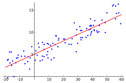
Linear regression will exist discussed in greater detail every bit we move through the modeling process.

For our dependent variable nosotros'll utilize housing_price_index (HPI), which measures price changes of residential housing.

For our predictor variables, nosotros use our intuition to select drivers of macro- (or "big picture") economic action, such as unemployment, involvement rates, and gross domestic product (total productivity). For an caption of our variables, including assumptions about how they impact housing prices, and all the sources of data used in this postal service, run across here.

Before anything, allow's go our imports for this tutorial out of the way.

The kickoff import is just to change how tables appear in the accompanying notebook, the rest will be explained in one case they're used:

            from IPython.display import HTML, brandish  import statsmodels.api as sm from statsmodels.formula.api import ols from statsmodels.sandbox.regression.predstd import wls_prediction_std  import matplotlib.pyplot equally plt import seaborn as sns %matplotlib inline sns.set_style("darkgrid")  import pandas as pd import numpy equally np          

You can grab the data using the pandas read_csv method directly from GitHub. Alternatively, you can download information technology locally.

            root = 'https://raw.githubusercontent.com/LearnDataSci/article-resources/master/Housing%20Price%20Index%20Regression'  housing_price_index = pd.read_csv(root + '/monthly-hpi.csv') unemployment = pd.read_csv(root + '/unemployment-macro.csv') federal_funds_rate = pd.read_csv(root + '/fed_funds.csv') shiller = pd.read_csv(root + '/shiller.csv') gross_domestic_product = pd.read_csv(root + '/gross domestic product.csv')          

One time we have the data, invoke pandas' merge method to bring together the data together in a unmarried dataframe for assay. Some information is reported monthly, others are reported quarterly. No worries. We merge the dataframes on a certain column so each row is in its logical identify for measurement purposes. In this case, the best column to merge on is the engagement column. See below.

            # merge dataframes into unmarried dataframe past engagement df = (shiller.merge(housing_price_index, on='date')                     .merge(unemployment, on='engagement')                     .merge(federal_funds_rate, on='date')                     .merge(gross_domestic_product, on='appointment'))          

Allow'due south get a quick look at our variables with pandas' head method. The headers in bold text correspond the date and the variables nosotros'll exam for our model. Each row represents a different fourth dimension period.

	engagement	sp500	consumer_price_index	long_interest_rate	housing_price_index	total_unemployed	more_than_15_weeks	not_in_labor_searched_for_work	multi_jobs	leavers	losers	federal_funds_rate	total_expenditures	labor_force_pr	producer_price_index	gross_domestic_product
0	2011-01-01	1282.62	220.22	iii.39	181.35	16.ii	8393	2800	6816	6.v	sixty.1	0.17	5766.vii	64.2	192.7	14881.3
ane	2011-04-01	1331.51	224.91	3.46	180.80	xvi.1	8016	2466	6823	6.viii	59.4	0.ten	5870.viii	64.2	203.1	14989.six
2	2011-07-01	1325.xix	225.92	3.00	184.25	15.9	8177	2785	6850	6.8	59.two	0.07	5802.6	64.0	204.6	15021.1
3	2011-x-01	1207.22	226.42	2.15	181.51	15.eight	7802	2555	6917	8.0	57.9	0.07	5812.nine	64.ane	201.1	15190.3
4	2012-01-01	1300.58	226.66	1.97	179.13	15.2	7433	2809	7022	7.4	57.one	0.08	5765.seven	63.vii	200.7	15291.0

Usually, the adjacent stride later gathering data would exist exploratory analysis. Exploratory analysis is the part of the process where we clarify the variables (with plots and descriptive statistics) and figure out the best predictors of our dependent variable.

For the sake of brevity, we'll skip the exploratory analysis. Keep in the back of your mind, though, that information technology'southward of utmost importance and that skipping information technology in the real globe would preclude ever getting to the predictive section.

We'll use ordinary to the lowest degree squares (OLS), a bones yet powerful way to assess our model.

OLS measures the accurateness of a linear regression model.

OLS is congenital on assumptions which, if held, bespeak the model may exist the right lens through which to interpret our data. If the assumptions don't hold, our model's conclusions lose their validity.

Take extra attempt to cull the right model to avert Car-esotericism/Rube-Goldberg's Disease.

Hither are the OLS assumptions:

1. Linearity: A linear human relationship exists betwixt the dependent and predictor variables. If no linear relationship exists, linear regression isn't the correct model to explicate our data.
2. No multicollinearity: Predictor variables are not collinear, i.e., they aren't highly correlated. If the predictors are highly correlated, try removing one or more of them. Since boosted predictors are supplying redundant data, removing them shouldn't drastically reduce the Adj. R-squared (see below).
3. Goose egg conditional mean: The average of the distances (or residuals) between the observations and the trend line is zero. Some volition be positive, others negative, merely they won't exist biased toward a set of values.
4. Homoskedasticity: The certainty (or doubtfulness) of our dependent variable is equal beyond all values of a predictor variable; that is, there is no pattern in the residuals. In statistical jargon, the variance is constant.
5. No autocorrelation (series correlation): Autocorrelation is when a variable is correlated with itself across observations. For case, a stock price might exist serially correlated if one day's stock price impacts the next solar day's stock price.

Permit's begin modeling.

Simple linear regression uses a unmarried predictor variable to explain a dependent variable. A simple linear regression equation is as follows:

$$y_i = \alpha + \beta x_i + \epsilon_i$$

Where:

$y$ = dependent variable

$\beta$ = regression coefficient

$\alpha$ = intercept (expected mean value of housing prices when our independent variable is zippo)

$x$ = predictor (or independent) variable used to predict Y

$\epsilon$ = the error term, which accounts for the randomness that our model tin can't explain.

Using statsmodels' ols role, we construct our model setting housing_price_index as a function of total_unemployed. Nosotros assume that an increase in the total number of unemployed people volition take downward force per unit area on housing prices. Perhaps we're incorrect, but we have to starting time somewhere!

The code beneath shows how to set up a simple linear regression model with total_unemploymentas our predictor variable.

            # fit our model with .fit() and show results # we use statsmodels' formula API to invoke the syntax below, # where we write out the formula using ~ housing_model = ols("housing_price_index ~ total_unemployed", data=df).fit()  # summarize our model housing_model_summary = housing_model.summary()  # convert our tabular array to HTML and add colors to headers for explanatory purposes HTML( (housing_model_summary     .as_html()     .supercede('<th>  Adj. R-squared:    </th>', '<thursday style="background-color:#aec7e8;"> Adj. R-squared: </th>')     .replace('<th>coef</th>', '<thursday style="background-color:#ffbb78;">coef</th>')     .supplant('<th>std err</thursday>', '<thursday mode="background-color:#c7e9c0;">std err</thursday>')     .supersede('<th>P>|t|</th>', '<th mode="background-color:#bcbddc;">P>|t|</th>')     .supplant('<th>[0.025</th>    <thursday>0.975]</th>', '<th fashion="groundwork-color:#ff9896;">[0.025</th>    <thursday style="background-color:#ff9896;">0.975]</th>')) )          

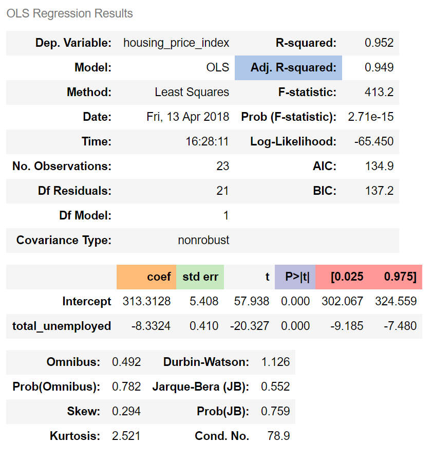
Outcome:

To explicate:

Adj. R-squared indicates that 95% of housing prices tin be explained by our predictor variable, total_unemployed.

The regression coefficient (coef) represents the change in the dependent variable resulting from a one unit change in the predictor variable, all other variables being held constant. In our model, a ane unit increase in total_unemployed reduces housing_price_index past 8.33. In line with our assumptions, an increment in unemployment appears to reduce housing prices.

The standard mistake measures the accurateness of total_unemployed's coefficient past estimating the variation of the coefficient if the same test were run on a different sample of our population. Our standard error, 0.41, is low and therefore appears authentic.

The p-value means the probability of an 8.33 subtract in housing_price_index due to a one unit increase in total_unemployed is 0%, assuming at that place is no relationship between the two variables. A low p-value indicates that the results are statistically significant, that is in general the p-value is less than 0.05.

The confidence interval is a range within which our coefficient is probable to fall. We can be 95% confident that total_unemployed'due south coefficient will be inside our confidence interval, [-nine.185, -seven.480].

Please see the four graphs below.

1. The "Y and Fitted vs. X" graph plots the dependent variable confronting our predicted values with a confidence interval. The inverse relationship in our graph indicates that housing_price_index and total_unemployed are negatively correlated, i.east., when ane variable increases the other decreases.
2. The "Residuals versus total_unemployed" graph shows our model'southward errors versus the specified predictor variable. Each dot is an observed value; the line represents the mean of those observed values. Since there's no pattern in the altitude between the dots and the mean value, the OLS supposition of homoskedasticity holds.
3. The "Partial regression plot" shows the relationship between housing_price_index and total_unemployed, taking in to account the bear upon of adding other contained variables on our existing total_unemployed coefficient. We'll see later on how this aforementioned graph changes when we add together more variables.
4. The Component and Component Plus Residual (CCPR) plot is an extension of the partial regression plot, but shows where our trend line would lie after adding the impact of adding our other contained variables on our existing total_unemployed coefficient. More on this plot here.

            # This produces our iv regression plots for total_unemployed  fig = plt.figure(figsize=(15,8))  # pass in the model as the first parameter, and so specify the  # predictor variable we want to clarify fig = sm.graphics.plot_regress_exog(housing_model, "total_unemployed", fig=fig)          

RESULT:

The next plot graphs our trend line (green), the observations (dots), and our confidence interval (red).

            # predictor variable (x) and dependent variable (y) 10 = df[['total_unemployed']] y = df[['housing_price_index']]  # Think our confidence interval values # _ is a dummy variable since we don't actually use information technology for plotting merely need it as a placeholder # since wls_prediction_std(housing_model) returns 3 values _, confidence_interval_lower, confidence_interval_upper = wls_prediction_std(housing_model)  fig, ax = plt.subplots(figsize=(10,7))  # plot the dots # 'o' specifies the shape (circle), we tin can as well use 'd' (diamonds), 's' (squares) ax.plot(10, y, 'o', characterization="data")  # plot the trend line # g-- and r-- specify the colour to use ax.plot(ten, housing_model.fittedvalues, 'g--.', label="OLS")  # plot upper and lower ci values ax.plot(x, confidence_interval_upper, 'r--') ax.plot(x, confidence_interval_lower, 'r--')  # plot legend ax.legend(loc='best');          

Outcome:

Mathematically, multiple linear regression is:

$$Y = \beta_0 + \beta_1 x_1 + \beta_2 x_2 + ... + \beta_k x_k + \epsilon$$

We know that unemployment cannot entirely explicate housing prices. To get a clearer pic of what influences housing prices, nosotros add and test different variables and analyze the regression results to see which combinations of predictor variables satisfy OLS assumptions, while remaining intuitively highly-seasoned from an economic perspective.

We make it at a model that contains the post-obit variables: fed_funds, consumer_price_index, long_interest_rate, and gross_domestic_product, in addition to our original predictor, total_unemployed.

Adding the new variables decreased the impact of total_unemployed on housing_price_index. total_unemployed's touch is now more unpredictable (standard error increased from 0.41 to 2.399), and, since the p-value is higher (from 0 to 0.943), less likely to influence housing prices.

Although total_unemployed may be correlated with housing_price_index, our other predictors seem to capture more of the variation in housing prices. The existent-world interconnectivity among our variables can't be encapsulated by a simple linear regression lonely; a more than robust model is required. This is why our multiple linear regression model's results alter drastically when introducing new variables.

That all our newly introduced variables are statistically significant at the v% threshold, and that our coefficients follow our assumptions, indicates that our multiple linear regression model is better than our simple linear model.

The code beneath sets up a multiple linear regression with our new predictor variables.

            # once again, invoke statsmodel'due south formula API using the below syntax housing_model = ols("""housing_price_index ~ total_unemployed                                              + long_interest_rate                                              + federal_funds_rate                                             + consumer_price_index                                              + gross_domestic_product""", data=df).fit() # summarize our model housing_model_summary = housing_model.summary() HTML(housing_model_summary.as_html())          

RESULT:

Now permit's plot our partial regression graphs again to visualize how the total_unemployedvariable was impacted by including the other predictors. The lack of tendency in the fractional regression plot for total_unemployed (in the figure below, upper right corner), relative to the regression plot for total_unemployed (above, lower left corner), indicates that total unemployment isn't as explanatory equally the outset model suggested. We too see that the observations from the latest variables are consistently closer to the trend line than the observations for total_unemployment, which reaffirms that fed_funds, consumer_price_index, long_interest_rate, and gross_domestic_product do a improve task of explaining housing_price_index.

These partial regression plots reaffirm the superiority of our multiple linear regression model over our unproblematic linear regression model.

            # this produces our half dozen fractional regression plots  fig = plt.figure(figsize=(20,12)) fig = sm.graphics.plot_partregress_grid(housing_model, fig=fig)          

RESULT:

Nosotros have walked through setting up bones simple linear and multiple linear regression models to predict housing prices resulting from macroeconomic forces and how to assess the quality of a linear regression model on a bones level.

To exist sure, explaining housing prices is a hard problem. There are many more predictor variables that could be used. And causality could run the other way; that is, housing prices could be driving our macroeconomic variables; and even more circuitous withal, these variables could be influencing each other simultaneously.

I encourage y'all to dig into the data and tweak this model past adding and removing variables while remembering the importance of OLS assumptions and the regression results.

Most importantly, know that the modeling process, being based in science, is as follows: test, analyze, fail, and test some more than.

This post is an introduction to basic regression modeling, but experienced information scientists will find several flaws in our method and model, including:

• No Lit Review: While it's tempting to dive in to the modeling process, ignoring the existing body of noesis is perilous. A lit review might have revealed that linear regression isn't the proper model to predict housing prices. It also might have improved variable selection. And spending time on a lit review at the outset can save a lot of time in the long run.
  
• Modest sample size: Modeling something as complex equally the housing market requires more than vi years of data. Our minor sample size is biased toward the events after the housing crisis and is not representative of long-term trends in the housing market.
  
• Multicollinearity: A careful observer would've noticed the warnings produced by our model regarding multicollinearity. Nosotros take two or more variables telling roughly the same story, overstating the value of each of the predictors.
  
• Autocorrelation: Autocorrelation occurs when past values of a predictor influence its current and hereafter values. Careful reading of the Durbin-Watson score would've revealed that autocorrelation is nowadays in our model.

In a hereafter mail service, we'll attempt to resolve these flaws to better understand the economic predictors of housing prices.

claxtonlareed.blogspot.com

Source: https://www.learndatasci.com/tutorials/predicting-housing-prices-linear-regression-using-python-pandas-statsmodels/

Share this post